Beryllium and Climate

 

Beryllium and Climate

John Reid

Abstract

Antarctic ice core proxy temperature variations are compared with insolation values at 60° N for the last 500 kyr. Linear regression shows that the insolation accounts for less than 10 percent of the variance of the temperature. The temperature exhibits a power law variance spectrum with an index of -2 implying that variations are the outcome of an integrating process such as a random walk. Significant peaks occur at obliquity and precession frequencies but none at the eccentricity frequency, below which there is a significant low frequency trough or cut-off. Comparison of the GISP2 10Be flux with GISP2 temperature variations suggest that different mechanisms underlie Dansgaard-Oeschger events, the Younger Dryas and Termination I. A model of ice age climate variations is proposed whereby the climate alternates between two metastable states.

Introduction

The idea that orbital changes cause variations in solar insolation which gives rise, in turn, to observed climate variations on a time scale of 10 to 100 kyr has dominated thinking in this field since early last century. More recently some workers have voiced reservations about whether such a mechanism can fully account for observed paleoclimate data; (see for example, Wunsch, [2004] and references therein). Clearly there is an orbital “signal” in the proxy temperature record [e.g. Kawamura et al, 2007]. Is this signal the sole, or even the major, cause of ice age temperature variations?

The causal link between orbital variations and ice core proxy temperatures is commonly assumed to be variations in solar insolation and the consequent expansion / contraction of the northern ice sheet. Hence Huybers [2006] has examined forcing due to insolation variations at 65°N. However there remain quasi-random temperature excursions known as Dansgaard-Oeschger events which do not quite fit this picture [Jouzel, 2007]

Underpinning these issues is the question of whether a particular time series is deterministic or stochastic or a mixture of the two. While it can never be possible to prove that any finite sequence of observations is either one or the other, statistical methods may be used to ascertain whether a deterministic signal is present at a given level of significance. This can be done by computing a variance spectral estimate and testing individual peaks and troughs within this spectral estimate for significance.

Time Series

EPICA Dome C data derived from EPICA Dome C ice cores [Jouzel et al, 2007] covering the period from 500 kyr to the present were examined. Earlier data were ignored because of lower sampling rates and because the obvious discontinuity which occurred at the Mid-Pleistocene Revolution [Maslin and Ridgewell, 2005] near 600 kyr bp precludes any assumption of stationarity prior to that time.

Figure 1: Smoothed and averaged EPICA Dome C data derived from EPICA Dome C ice cores (black) and computed integrated insolation energy values for Latitude 60o North and threshold insolation 275 w/m2 due to Huybers and Eisenman (red). The time series of residuals after subtracting the predicted values is also shown (grey).

By definition a time series comprises a sequence of quantities sampled at equal intervals of time. Typically, as a result of ice flow behaviour, more recent ice core data from near the surface is sampled much more densely in time than is deeper, older data. Time series were constructed by partitioning the data into sampling intervals of equal length. The values of all the data points lying within each sampling interval were then averaged and the mean assigned to the mid-time of that sampling interval. Where no data points occurred within an interval, the closest was chosen. For spectral analysis purposes the time interval was chosen as 0.125 kyr with 4096 samples spanning the period from the present to 512 kyr ago. For regression purposes 500 sampling intervals were chosen each of 1kyr in length and spanning the period from the present to 500 kyr ago.

The time series derived in this way is shown as the middle curve in Figure 1. Also shown in Figure 1 as the lower, red curve is the time series of computed integrated insolation energy values for Latitude 60o North and threshold insolation 275 w/m2 due to Huybers and Eisenman [2006].

Variance Spectra

Each ordinate of the periodogram of a white noise process divided by the population value has a chi-squared distribution with two degrees of freedom whatever the length of the sequence may be. If the periodograms of a number of data sequences of the same length, sampled from the same population are averaged, as in Bartlett’s method, then the mean periodogram tends to the population value as the number sampled tends to infinity, i.e. the periodogram is a consistent estimate when looked at as a special case of Bartlett’s method.

Insolation is computed from the equations of celestial mechanics and so is deterministic. Its population spectrum will therefore comprise delta functions corresponding to each of the sinusoids present. Hence in detecting the presence of an insolation signal in ice-core variance spectra we need to look for spectral lines, i.e. for concentrations of variance in very narrow frequency intervals. For this reason the un-windowed periodogram is the most appropriate spectral method to use in this case because it is the consistent spectral estimate with the best frequency resolution. Numerical experiments using Bartlett’s and Welch’s methods by So et al [1999] confirm that the simple periodogram gives optimum spectral performance in detecting a sinusoid in white noise.

The variance density spectral estimates for the two time series shown in Figure 1 are shown plotted using logarithmic scales in Figure 2. Each spectral estimate is the squared modulus of the Fourier transform of the time series. No smoothing or windowing was carried out in either the time domain or the frequency domain. The spectral estimates at frequencies near the Nyquist frequency (4 kyr-1) are distorted by aliasing and are not shown.

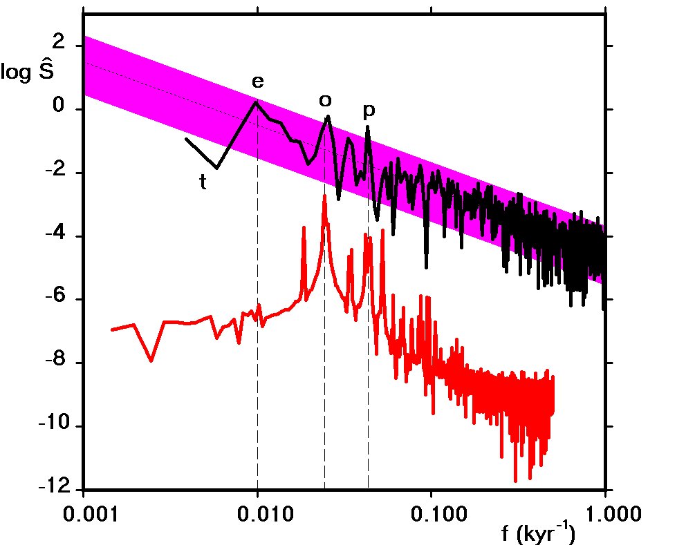
Figure 2: The variance density spectral estimates of the time series shown in Figure 1 (black: data, red: insolation). The dotted line shows the locus of an spectrum and the magenta band the 95% confidence limits about this locus. Peaks in the insolation spectra due to eccentricity, obliquity and precession at .01, .0244 and .043 kyr-1 are shown by the vertical dashed lines labeled a, b and c respectively.

In Figure 2,. frequencies of important peaks in the insolation spectra are shown by the vertical dashed lines labeled a, b and c, the frequencies due to the eccentricity, obliquity and precession of the earth in its orbit respectively.

A regression analysis of against gave a value for the slope of the line of best fit as . The dotted line in Figure 2 shows the locus of an spectrum. The magenta band shows the upper and lower 95% confidence limits derived from the null hypothesis that is a constant, whereis the population variance density at frequency, , i.e. that the first differences of the temperature time series comprises un-self-correlated (“white”) noise. Thus around 5% of the spectral estimate values should lie outside the confidence limits by chance alone.

Nevertheless the obliquity and precession peaks at b and c are significant (P = .003 and .0002 respectively), indicating the presence of these orbital components in the variance spectrum. More importantly the eccentricity peak, a, is not significant at all, while there is a significant trough at lower frequencies, i.e. there is a significant (P = .01) low frequency cut-off as discussed by Wunsch [2003].

The power law is strong evidence for the sort of climate random walk first proposed by Hasselmann [1976]. The existence of such a power-law also strongly implies that the population spectrum is a continuum and so the outcome of a stochastic process.

Huybers and Curry [2006] carried out a similar search for power law scaling using a wide variety of instrumental and proxy records. They found red spectra but with smaller absolute indices. They did not attempt to fit a power law locus in the 100 kyr to 1 kyr range as was done here. Had they done so their Figure 2 indicates that they too would have found an inverse square power law in this range.

Linear Regression of Time Series

The assumption that proxy temperature, , is driven primarily by Northern Hemisphere insolation can also be tested by performing a linear regression analysis of values as the dependant variable against insolation values. 500 sample pairs were used. The sample correlation coefficient, , was .305. Thus , the fraction of variance accounted for by the insolation values, was .093, i.e. just under 10% as previously determined by Wunsch [2004].

The sequence of residuals is also plotted in Figure 1 (grey, top). All of the major features present in the record remain in the sequence of residuals. Note however that the sequence of residuals is uncorrelated with the insolation values as a consequence of the regression process. Numerous insolation series are provided online by Huybers and Eisenman for different latitudes and threshold values. The regression process was carried out for each of these and most gave very similar results. The Latitude (60° N) and the insolation threshold of 275 w/m2 were chosen because they gave the highest correlation value. Vostok data also yielded a similar correlation coefficient (r = 0.242, r2 = .059).

Nevertheless, this cannot be the whole story. Kawamura et al [2007] using a new technique involving the trapped N2/O2 ratio to fix summer insolation values experimentally, have shown that the last four terminations have occurred at times of increasing Northern Hemisphere insolation implying that insolation must be involved somehow even if only as a trigger or an “enabling switch”.

Even so, it should be noted that terminations do not occur on every occasion that insolation conditions are favorable but sometimes every 2nd time and sometimes every 3rd time. This too implies that the underlying mechanism is primarily stochastic but is modulated to some extent by insolation forcing.

Beryllium 10 flux

Beryllium 10 is produced in the stratosphere by collision of cosmic rays with atmospheric particles. Its production rate is therefore controlled by the primary cosmic ray intensity, by solar modulation and by geomagnetic modulation, all of which processes lie outside of the climate system. Within the climate system, the accumulation rate within the cored sample may be modulated by the rate at which 10Be moves latitudinally and from the stratosphere to the troposphere and into the snow itself and by the rate of snow accumulation or “dry” precipitation. These effects have been modeled by a number of workers [e.g., Kovaltsov and Usoskin, 2010 and Heikkilä et al, 2011] and climatic effects observed experimentally by Pedro et al [2006]. Field et al [2006] using a GCM have demonstrated the possibility of significant climate related variation in 10Be flux rate. At issue is whether observed variations in the 10Be flux rate are indicative of external forcing of climate or merely passive markers of upheavals internal to the climate system.

Figure 3: Raw 10Be flux (red) calculated by multiplying the 10Be concentration in GISP2 ice by the corresponding GISP2 accumulation rate. Also shown is the GISP2 Ice Core Temperature (blue, bottom curve) and EPICA Dome C (black, top curve) for the same period. The 10Be flux is plotted upside down for ease of comparison with the other curves.

Figure 3 shows the raw 10Be flux (red) calculated by multiplying the 10Be concentration in GISP2 ice, 719 – 2253 m [Finkel and Nishiizumi, 1997] by the corresponding GISP2 accumulation rate [Alley, 2000, 2004]. Also shown (blue, bottom curve) is the GISP2 Ice Core Temperature [Alley, 2000, 2004] and EPICA Dome C (top curve) for the same period. The temperature data were sampled as described above with a sampling interval of 0.1 kyr. Note that the 10Be flux values were not smoothed and are plotted upside down for ease of comparison with the other two time series. Beryllium data is available from other sites such as NGRIP and Taylor Dome but the GISP2 data was more closely sampled in time and had the added advantage that accumulation rate data obtained from the same cores were available.

The data plotted in Figure 3 imply that there are three different types of temperature variation event:

Firstly, in the range 25 kyr to 40 kyr there is a strong resemblance between the GISP2 temperature data and the 10Be flux, with 7 peaks in the temperature corresponding closely to 7 depressions in the 10Be flux. These excursions in temperature are known as Dansgaard-Oeschger events [see, e.g. Dansgaard et al, 1993]. They are present, but are much less pronounced, in the Southern Hemisphere, EPICA, temperature data as noted by Jouzel et al [2007].

Secondly, the 10Be flux exhibits both a peak and a trough near 13.5 kyr bp An increase in 10Be flux was followed by a decrease, corresponding to the onset and decay of the temperature excursion known as the Younger Dryas [Alley, 2000].

Thirdly, the most prominent feature in the ice core temperature record of the last 40 kyr, Termination I, which occurred 11 kyr ago, shows no corresponding excursion in the 10Be flux record.

Discussion

Wunsch [2004] fitted an AR(2) process to Vostok temperature data and found the innovation or forcing sequence contains impulses in the form of short runs of positive values corresponding to times of rapid deglaciation, i.e. to terminations. This corresponds to the observation that deglaciation proceeds much more rapidly than glaciation, i.e. that there is a time asymmetry in the temperature record: rapid onset is followed by slow decay. The temperature variance spectrum displayed in Figure 2 tells us nothing about the distribution of the innovation; all it tells us is that uncorrelated noise has been passed through an integrator such as an RC circuit in electronics. A sequence of discrete random impulses will do just as well as Gaussian white noise. Indeed, the fact that these termination-related impulses are not completely random but are separated by multiples of approximately 40 kyr is the reason for the 40 kyr peak, peak b in Figure 2. The random walk hypothesis of Hasselmann [1976] still applies but instead of a Gaussian white noise process due to weather, terminations appear to be forced by discrete impulses which occurred about 80 or 120 kyr apart, after each of which the climate relaxed exponentially back to its prior, ice age state. It is this exponential decay which leads to the power law of Figure 2.

There are two possible models for ice ages and their terminations, viz.: an external model under which some external forcing such as increased solar activity pushes the earth’s climate out of its usual ice age state, and, an internal model under which the earth’s climate has two metastable states and alternates between them spontaneously with little or no external forcing.

The second model is more likely for two reasons: (1) the most recent termination was accompanied by no significant change in the GISP2 10Be flux implying that nothing unusual was happening elsewhere in the solar system at the time, and (2) the last four terminations occurred at times of increasing insolation [Kawamura et al, 2007] suggesting that mild heating of the northern polar cap was all that was necessary to trigger the catastrophic collapse of the ice age metastable state.

The low frequency cut-off, the significant reduction in variance density at frequencies below 0.01 kyr-1 evident in Figure 2, is relevant here. This is manifested in the time domain by the regularity of the maximum temperatures achieved during interglacials and of the minimum temperatures achieved during ice ages. There is little long-term drift or cyclic trend. Thetime series of Figure 1 resembles the output of an electronic circuit known as multivibrator which is forced by positive feedback to oscillate noisily between two extreme metastable states. In the case of a climate oscillator these two states could be the high greenhouse gas / low ice albedo state of the interglacials and the low greenhouse gas / high ice albedo state of the ice ages.

No explanation can be offered for Dansgaard-Oeschger events which appear to be unrelated to this mechanism. The fact that, unlike insolation changes, DO events do not trigger terminations suggests that they are more local in character.

References

Alley, R.B. (2004), GISP2 Ice Core Temperature and Accumulation Data, IGBP PAGES/World Data Center for Paleoclimatology – Data Contribution Series #2004-013.
NOAA/NGDC Paleoclimatology Program, Boulder CO, USA.

Alley, R.B. (2000), The Younger Dryas cold interval as viewed from central Greenland, Quaternary Science Reviews, 19, 213-226.

Dansgaard, W., S. J. Johnsen, H. B. Clausen, D. Dahl-Jensen, N. S. Gundestrup, C. U. Hammer, C. S. Hvidberg, J. P. Steffensen, A. E. Sveinbjörnsdottir, J. Jouzel and G. Bond (1993), Evidence for general instability of past climate from a 250-kyr ice-core record, Nature 364 (6434), 218–220, doi:10.1038/364218a0.

Field, C.V., G.A. Schmidt, D. Koch, and C. Salyk (2006), Modeling production and climate-related impacts on 10Be concentration in ice cores, J. Geophys. Res., 111, D15107, doi:10.1029/2005JD006410.

Finkel, R.C., and K. Nishiizumi (1997), Beryllium 10 concentrations in the Greenland Ice Sheet Project 2 ice core from 3-40 ka, J. Geophys. Res., 102, 26699-26706.

Hasselmann, K. (1976), Stochastic climate models, Part I, Theory, Tellus, XXVIII, 6.

Heikkilä U., J. Beer, J.A. Abreu and F. Steinhilber (2011), On the Atmospheric Transport and Deposition of the Cosmogenic Radionuclides (10Be): A Review, Space Science Reviews, doi: 10.1007/s11214-011-9838-0.

Huybers, P. and W. Curry (2006), Links between annual, Milankovitch and continuum temperature variability, Nature, 441(7091), 329-332.

Huybers, P. and I. Eisenman, (2006). “Integrated Summer Insolation Calculations”. IGBP PAGES/World Data Center for Paleoclimatology, Data Contribution Series # 2006-079. NOAA/NCDC Paleoclimatology Program, Boulder CO, USA.

Jouzel, J., V. Masson-Delmotte, O. Cattani, G. Dreyfus, S. Falourd,
G. Hoffmann, B. Minster, J. Nouet, J.M. Barnola, J. Chappellaz, H. Fischer,
J.C. Gallet, S. Johnsen, M. Leuenberger, L. Loulergue, D. Luethi, H. Oerter,
F. Parrenin, G. Raisbeck, D. Raynaud, A. Schilt, J. Schwander, E. Selmo,
R. Souchez, R. Spahni, B. Stauffer, J.P. Steffensen, B. Stenni, T.F. Stocker,
J.L. Tison, M. Werner, and E.W. Wolff. (2007), Orbital and Millennial Antarctic Climate Variability over the Past 800,000 Years, Science, 317(5839),793-797.

Kawamura, K., F. Parrenin, L.Lisiecki, R. Uemura, F. Vimeux, J.P. Severinghaus, M.A.Hutterli, T. Nakazawa, S. Aoki, J.Jouzel, M.E. Raymo, K. Matsumoto, H. Nakata, H. Motyama, S. Fujita, K. Goto-Azuma, Y. Fujii and O. Watanabe. (2007), Northern Hemisphere forcing of climatic cycles in Antarctica over the past 360,000 years, Nature 448(0615), 912-916.

Kovaltsov, G.A. and I.G. Usoskin (2010), A new 3D numerical model of cosmogenic nuclide 10Be production in the atmosphere, Earth and Planetary Science Letters, 291, 182-188, doi:10.1016/j.epsl.20010.01.011.

Maslin, M.A. and A.J. Ridgwell (2005), Mid-Pleistocene Revolution and the “eccentricity myth”, Geological Society, London, Special Publications, 247,19-34.

Pedro, J.B., T.D. van Ommen, M.A.J. Curran, V.I. Morgan, A. Smith and A.J. McMorrow (2006), Evidence for climate modulation of the 10Be solar activity proxy, J. Geophys. Res., 111(21), 1-6, doi:10.1029/2005JD006764.

So, H.C. , Y. T. Chan , Q. Ma and P. C. Ching (1999), Comparison of Various Periodograms for Sinusoid Detection and Frequency Estimation, IEEE Trans. Aerospace Electronic Systems. 35(3), 945-951.

Wunsch, C. (2003), The spectral description of climate change including the 100 ky energy, Climate Dynamics, 20, 353-363, doi 10.1007/s00382-002-0279-z.

Wunsch, C. (2004), Quantitative estimate of the Milankovitch-forced contribution to Quaternary climate change, Quaternary Science Reviews, 23,1001-1012, doi:10.1016/j.quascirev.2004.02.014.