

Local Climate Sensitivities estimated from HadCRUT temperatures and CO2 concentrations using the ARX method. They are rounded to the nearest integer for display purposes. ( Figure 5 of my recent paper submitted to Proceedings of the Royal Society: A. )
Figure 5 is overwhelming evidence that CO2 does force temperature . No modeller has come up with anything close to Figure 5, because numerical models are just not good enough. They give a reasonable estimate of global climate sensitivity because they have been tweaked to do that.
I recently found that someone else has used statistical methods to map local climate sensitivity.

(Asinimov, O. A. (2001).”Predicting Patterns of Near-Surface Air Temperature Using Empirical Data”, Climatic Change 50: 297-315).
The is a striking resemblance to my Figure 5 above, particularly with regard to high values in Siberia and NW Canada.
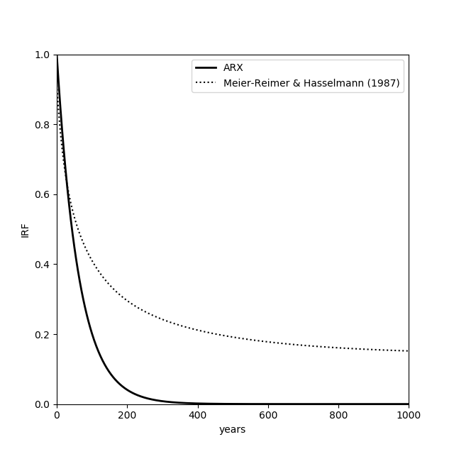
Figure 3 shows that numerical model estimates of the long-term rate of removal of atmospheric carbon are hopelessly wrong (but politically correct). In fact, half of the CO2 in the atmosphere is removed every 43 years.
Download preprint: Reid2022
Publication History
I originally submitted to PNAS who replied :
… This decision is necessarily subjective and does not reflect an evaluation of the technical quality of your work or of its appropriateness for a more specialized audience.
Thank you for submitting your work to PNAS; we wish you success in finding a more suitable venue for publication soon.
Proc. Roy Soc. A were not so kind. Evidently the paper is marred by its simplicity:
The author applied a statistical method to some climate time series and the conclusions are useful and consistent with what is already known. However, the statistical method is too simple and cannot provide relevant new insights into such a complex problem as climate change.
This encapsulates the anti-empirical head-set of the Climate Change industry: “I have made up my mind. Don’t confuse me with facts.” Ever heard of Occam’s Razor?
Although some conclusions can be drawn from the performed analysis, the causality of the conclusions is doubtful.
Easily fixed. The next iteration of the paper will include a section on Granger Causality which is well suited to the ARX methodology.
The paper raises an interesting question about the long term retention of CO2 in the atmosphere, in contrast to the result of an earlier publication. In future work I suggest that the author needs to establish more clearly why his result on the question of atmospheric retention of CO2 differs from that of Reference 11
Reference 11 is to Meier-Reimer and Hasselmann (1987) and we are talking about Figure 3 above. I did in fact establish why my result differs from theirs in the conclusion section, viz.:
A possible explanation is the following. The deep ocean is bounded by a turbulent mixed layer and by the highly turbulent Antarctic Circumpolar Current. It is therefore likely to be internally mixed by a Kolmogorov cascade of turbulent eddies, some with spatial scales as large as ocean basins and with time scales of, perhaps, decades. Turbulence is a stochastic phenomenon which is difficult to observe at large spatial and temporal scales and which, being stochastic, cannot be readily emulated by deterministic models such as OAGCMs. Eddy diffusion generated by turbulent mixing would greatly increase the capacity of the deep ocean to absorb carbon dioxide and so could account for the shorter half time of the observed impulse response of atmospheric CO2 concentration. Whatever the explanation, there is no evidence for the long half times and remnant component of atmospheric CO2 concentration in , presently assumed by most modellers.
I can only assume that the Editor had either not read that paragraph, or, having done so, had not understood it. Ideally the paper should have been reviewed by at least one person who could actually understand it.
It’s called “peer review”.
One thing that, as a non-scientist, has always concerned me about the climate debate is the constant negativity about it. Alarmism at its worst.
There are entire countries in Africa that grow more food than they have for centuries, possibly ever. We have fewer famines. On a world-wide basis, people are better fed than they’ve ever been in the entire course of human history.
I blame activist scientists and the media. Many of the former have based their entire careers on a discipline for which funding will only continue as long as people are worried. (I don’t see how you can be an activist and scientifically objective at the same time.) Many of the latter, journalists and editors, seem to regard it as their moral duty to whip up as much hysteria as possible, witness COVID.
Wow!. That is a tour de force John. I am impressed.
I am not sure what to do next. I am thinking of looking at specific localities in more detail. e.g. the place in Northern Siberia (not shown) where the Climate Sensitivity is 12. Probably just bad data but who knows? It should also be possible to distinguish between CO2-related changes and changes due to other causes.
I am amazed at how good this method is. Why wasn’t this done 40 years ago? I suspect it is because, as soon as someone comes up with a new statistical technique, it is tried out in Econometrics where most of the cutting edge stats is published (and where there might be $$$ in it). This ARX technique may not work so well in Econometrics. It works for climate because it describes diffusion so well. The underlying “physics” in Econometrics may not be so tractable.
Hi John,
Strategically, in regard to the Royal Society, what I’d do is write a paper designed specifically just to get publshed. Remember the audience is not the reader but the Academy. Write as esoteric and arcane as all hell, suck up to them, forget about trying too hard to make your point (but make a point of course).
Your comment, “Easily fixed. The next iteration of the paper will include a section on Granger Causality which is well suited to the ARX methodology,” shows the trap you are in, trying to stick it to them, they who cannot be stuck. Be cleverer.
Once you have one with them, the others should be easier for them to accept with that precedence. Then do the real piece.
Good luck and good work.
Thanks Allan. One can only go so far in “sucking-up” although I could perhaps have left out the bit about the shorter half-life of atmospheric CO2.
Yes, my comment was a bit Rumpole of the Bailey-ish.
You’re not the first, John, to suffer injustice. This was just as bad. Skip to the middle, say 1:00:00, if you find the start too slow : https://www.youtube.com/watch?v=VYDaqto22NY
That fluidity is fundamentally granular, as John has long been arguing, has recently been demonstrated by Quantum Mechanics researchers, without their being aware of this
(because NOT wanting to, their sticking to their specialty, their wanting to stay there) :
The five grey crosses mentioned under Figure 1e in the article link below by these people, are explained in these terms :
“The magnification reveals vortex streets between adjacent droplets (grey crosses), indicating counterflow at their interface”.
They also clearly show the Classical to Quantum transition that John has been alluding to, strongly indicated by the Kolmogorov eddy cascade which is otherwise difficult to explain AND is also well illustrated by those five crosses, shown here as cascading all the way to Quantum bits, John’s granularity of fluids.
John has been facing two big barriers :
1. ) One of the first “scientists” John started criticizing was awarded a Nobel Prize last year, while ;
2.) One of the first equations John started to question were the Classical ~200 year old Navier–Stokes equations which Climate Catastrophe “scientists” hold close to their hearts, very much like those “Quantum Mechanics researchers [wanting to keep their careers]”, only more so, their being into much bigger money, heaps of it, from Western Governments.
The article :
https://www.nature.com/articles/s41586-021-04170-2.epdf?sharing_token=GyyjvNidJYV6fJeXAHmXCdRgN0jAjWel9jnR3ZoTv0O3HVFyXzlqYrpk-oqPk89HGVEDY1CeRClNxnX6Mw6OSpNQ3vpPADfZyQPWFTxep4VXnErj5b0Dyb5pqvzaEoZJ2G3z15HrvFWhLg187NiYbpw2bCLxD8UfM-uRp0NIZRByQjr6Nf8_w3MXw_iQFnflnHZkpctOcCIgZYcElFe21o0RYb9IjcfXywYDT9mxJnI%3D&tracking_referrer=arstechnica.com
Wow! So recognisable turbulence is observed in arcane states of matter such as the Bose-Einstein condensate. It seems the only substance in which turbulence does not occur then is a continuum, the state of matter described by the Navier-Stokes equations of fluid dynamics which is sometimes chaotic instead. Chaos is deterministic, turbulence is stochastic. No-one has ever observed chaos in the real world, it is a property of differential equations.
btw Peter is referring to https://www.amazon.com.au/Fluid-Catastrophe-John-Reid/dp/1527532062
Yes, the Quantum Mechanical foundational roots of turbulence is clearly demonstrated by this experimental observation of a Kolmogorov Eddy Cascade’s continuation into the Quantum conditions of a Bose-Einstein condensate from bigger eddies in a Classical State, thus proving that turbulence is indeed, purely and simply, one of an increasing class of macro phenomena that are entirely Quantum Mechanical, a class that already includes Super-Conductivity, Super-fluidity . . . with Chaos Theory having no place in their understanding.
Related : https://www.facebook.com/photo/?fbid=10211482205718386&set=a.10209900078246188
“… this page not available …”